Visualize Graphs from Adjacency Matrices

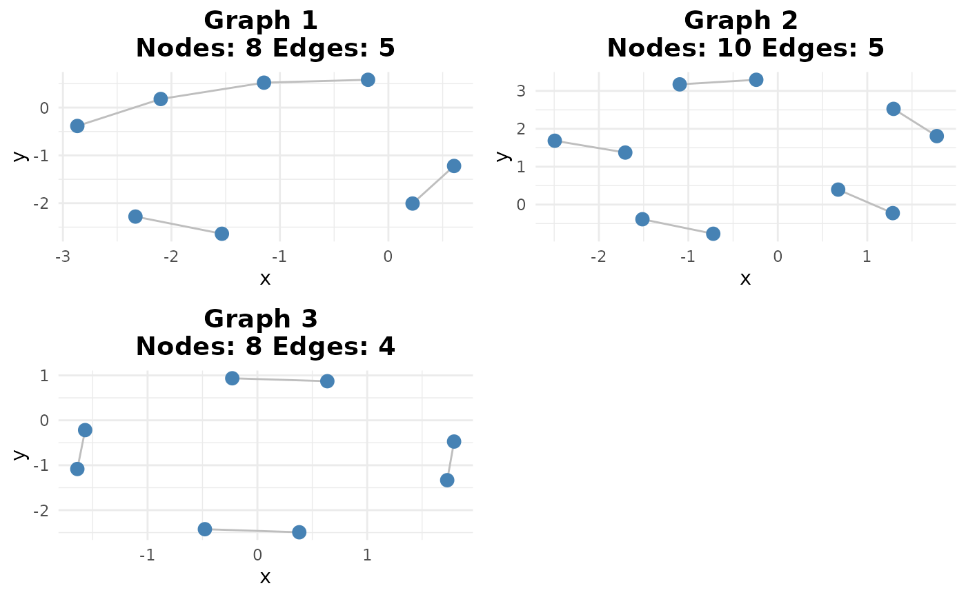
Generates and arranges multiple graph visualizations from a list of adjacency matrices. Each matrix is converted into an undirected igraph object and visualized using a force-directed layout via ggraph.

Usage

plotg(adj_matrix_list)

Arguments

adj_matrix_list

A list of square, symmetric adjacency matrices with zeros on the diagonal (no self-loops). Each matrix represents an undirected graph.

Value

A grid of plots displaying all valid graphs in the input list.

Details

Each adjacency matrix is validated to ensure it is square and symmetric. Disconnected nodes (degree zero) are removed prior to visualization. Graphs are visualized with a force-directed layout using ggraph, and multiple plots are arranged into a grid with gridExtra.

Each subplot title includes the graph index, number of nodes, and number of edges.

Note

This function requires the following packages: igraph, ggraph, and gridExtra. If any are missing, an informative error will be thrown.

Examples

data(count_matrices)

networks <- infer_networks(
    count_matrices_list = count_matrices,
    method = "GENIE3",
    nCores = 1
)
head(networks[[1]])
#>   regulatoryGene targetGene    weight
#> 1          HLA-A       CD74 0.2024512
#> 2          ARPC2      ARPC3 0.1894946
#> 3          ARPC3      ARPC2 0.1587442
#> 4           CD3E       CD3D 0.1536509
#> 5          HLA-E        FOS 0.1474853
#> 6         GNB2L1      UBA52 0.1452552

wadj_list <- generate_adjacency(networks)
swadj_list <- symmetrize(wadj_list, weight_function = "mean")

binary_listj <- cutoff_adjacency(
    count_matrices = count_matrices,
    weighted_adjm_list = swadj_list,
    n = 2,
    method = "GENIE3",
    quantile_threshold = 0.99,
    nCores = 1,
    debug = TRUE
)
#> [Method: GENIE3] Matrix 1 → Cutoff = 0.10949
#> [Method: GENIE3] Matrix 2 → Cutoff = 0.10210
#> [Method: GENIE3] Matrix 3 → Cutoff = 0.11277
head(binary_listj[[1]])
#>       ACTG1 ARPC2 ARPC3 BTF3 CD3D CD3E CD74 CFL1 COX4I1 COX7C CXCR4 EEF1A1
#> ACTG1     0     0     0    0    0    0    0    0      0     0     0      0
#> ARPC2     0     0     1    0    0    0    0    0      0     0     0      0
#> ARPC3     0     1     0    0    0    0    0    0      0     0     0      0
#> BTF3      0     0     0    0    0    0    0    0      0     0     0      0
#> CD3D      0     0     0    0    0    0    0    0      0     0     0      0
#> CD3E      0     0     0    0    0    0    0    0      0     0     0      0
#>       EEF1D EEF2 EIF1 EIF3K EIF4A2 FOS FTH1 FTL GNB2L1 HLA-A HLA-B HLA-C HLA-E
#> ACTG1     0    0    0     0      0   0    0   0      0     0     0     0     0
#> ARPC2     0    0    0     0      0   0    0   0      0     0     0     0     1
#> ARPC3     0    0    0     0      0   0    0   0      0     0     0     0     0
#> BTF3      0    0    0     0      0   0    0   0      0     0     0     0     0
#> CD3D      0    0    0     0      0   0    0   0      0     0     0     0     0
#> CD3E      0    0    0     0      0   0    0   0      0     0     0     0     0
#>       JUN JUNB MYL12B MYL6 NACA PABPC1 PFN1 TMSB4X UBA52 UBC
#> ACTG1   0    0      0    0    0      0    0      0     0   0
#> ARPC2   0    0      0    0    0      0    0      0     0   0
#> ARPC3   0    0      0    0    0      0    0      0     0   0
#> BTF3    0    0      0    0    0      0    0      0     0   0
#> CD3D    0    0      0    0    0      0    0      0     0   0
#> CD3E    0    0      0    0    0      0    0      0     0   0
plotg(binary_listj)